Time series modelling: Eclipsing binary stars
Eclipsing Binary Stars
Eclipsing binary stars are a benchmark in stellar astrophysics (check out this small blog post for some more about eclipsing binaries) - by modelling the time series signature of eclipses, we can obtain extremely high precision (<1%) inferences of fundamental stellar properties like their masses and radii. My work involves using a Markov Chain Monte Carlo procedure to model time series data of eclipsing binary stars to obtain inferences on the parameters of these models. In this post, we’ll go through what eclipsing binary stars are, and how we model them!
The data:
Almost all stars vary their brightness on some level if you look close enough. Using both ground based and space based satellites, we’ve managed to measure the brightness of stars in time on industrial scales. In astronomy, the resulting time series data are known as a lightcurve (yes, astronomers are very creative in their naming schemes).
In particular, space-based telescopes produce high quality time series of stars with a regular sampling of either 1, 2, or 30 minutes between consecutive observations. Thus, per object, we have a large quantity of high quality data to model! Despite this apparent blessing, there is a lot of potential for problems - specifically during data reduction. When going from raw photons collected on a CCD to a calibrated time series, we do a lot of processing that we often don’t care, or don’t want, to know about (think sausages). A perfect example of this is seen in the case of HD 165246 - an eclipsing binary with a pulsating O star primary and B type companion observed by the repurposed K2 mission.
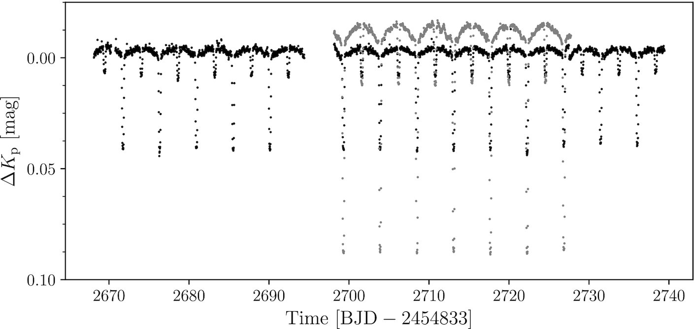
In this work, we investigated data that was reduced using two different methods. In the first method, we built a custom aperture by manually selecting the pixels that would be included in the mask when we construct the light curve. On the left, we see the red and blue outlines, representing the original algorithm selected mask (red) and the custom manually selected mask (blue). The second method uses a technique called Halo photometry, in which we use the scattered light on all pixels to construct a light curve - in effect, this mask is the inverse of the red profile on the left. This gives us two different time series to work with, shown below.
Bad data
Working with bad data is worse that working with no data because if we fit a model to the bad data and make decisions or statements based on the bad data, those statements won’t be worth very much. That’s why we have to understand what’s going on with our two different time series to the right. The time series obtained with method 1 is shown in black and with method 2 is shown in grey.
Immediately, we notice that the time series from method 2 is shorter (due to limitations from the halo photometry method) and it exists on an entirely different scale to the time series from method 1. This is because the halo photometry method introduces a large fraction of extra light into the data, which effectively dilutes our signal by increasing the noise level. Because of this, with our study we decided to use the black time series from method 1 to build our model.
The model - PHOEBE vs. ELLC
To model the eclipse signal in our time series data, we use two codes called PHOEBE and ELLC. These codes take a vector of input parameters θ and a time vector t and construct a mesh grid for each star (which allows it to be non-spherical), and then for each time tⱼthe algorithm calculates the visible surface of both stars, detects whether eclipses are occurring, and sums up the total light visible by an observer at some specified inclination and orientation to the binary system.
The two codes make different assumptions, use different numerical schemes, and take in different sets of input parameters - so when we use these, we want to make sure that the resulting physical parameters are the same - remember that we are interested in estimates for the masses and radii of the two stars.
Optimisation and results
Markov Chain Monte Carlo
We know the task - fit our model to the data and get inferences on the model parameters and physical properties of the stars. To do this, we’re going to use a method called Markov Chain Monte Carlo (MCMC) to explore the uncertainties on our model parameters and provide robust parameter inferences. In brief, MCMC is a method of numerically sampling the posterior distribution of our parameters as given by Bayes’ theorem (eqn. on the right), where θ is the vector of parameters that we want to obtain inferences for and d is the data. I’ll give a more detailed description of MCMC in a different post, but for this I’ll just say that I mostly use the emcee affine-invariant ensemble sampler for my codes, but there are plenty of other implementations.
In our case of HD 165246, we have to make some specific considerations. First, we are modelling two separate time series with one underlying model, and therefore, we have shared parameters that we need to sample jointly! The reason that we have two separate time series is that we are using both photometric time series data (the light curve seen above) and radial velocity time series data derived from spectroscopic measurements (seen to the right).
In this instance, the radial velocity data has information on the orbital separation and the ratio of masses of the two stars, while the eclipses in the photometry have information on the sizes and temperatures of the stars. Thus, to get a full model, we have to include both types of time series observations.
In total, our θ vector has 16 free parameters that we want inferences for.
Inferences and uncertainties
Two of the major motivations for using a Bayesian approach such as MCMC is that it i) allows us to incorporate outside information through the prior p(θ), and ii) it provides us with robust uncertainty estimates.
Through sampling, we build up a numerical approximation of the marginalised posterior distributions for each parameter (example for 4 parameters seen on the left). This gives us both a robust estimate of the parameter, as well as its distribution, which is immensely helpful for understanding how our model reproduces the data.
With this, we’re done! We have a set of optimal parameters for our model, given the data, and we have a distribution for each parameter so we know what range of values it can reasonably take. Although it kind of defeats the point, we can take the median of our marginalised posteriors and build the “optimal” model for our data (seen below as the solid black line). Furthermore, we can see that the fit is pretty good by investigating the residuals in the lower panel.
Code and method Comparisons
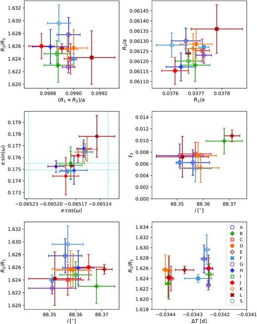
In reality, each binary star system has one set of values that describe the system and the stars that comprise it. In practice, however, there are many models and methods that can be used to estimate the true underlying values. In 2020, I was part of a study that used a well studied benchmark system AI Phe to compare different codes (including PHOEBE and ELLC) and methods for obtaining parameter inferences for eclipsing binary systems. While we all used the same data, in total, we used 13 different combinations of models, optimisation routines, and assumptions to model the data. In the end, we all produced remarkably similar results! The image on the right is a plot from the study where we plot the different parameter values and uncertainties obtained by the 13 different modelling approaches. If you look at the scale of the scatter, it is remarkably small.
What’s more is that when propagated into systematic uncertainties on the fundamental masses and radii of the stars, we find a systematic uncertainty of less than 0.1% in radius and 0.08 % in mass. This is an astounding result, which highlights the importance that eclipsing binaries hold in astrophysics as highly precise benchmarks for calibrating evolutionary models and theories.
Extensions and future work
Multiple sources of variability
While codes like PHOEBE and ELLC are great, the models don’t always capture all of the signal present in the data. For example, stars often exhibit multiple types of intrinsic variability such as spots, flares, or pulsations that further modulate the observed brightness in addition to the eclipses. This can often result in local minima when optimising our models or biased fits. To circumvent this, we can either i) use an iterative approach to model different sources of variability, or ii) model other signals simultaneously with a flexible model such as a Gaussian Process. More on that later!
Computational considerations
While MCMC is very useful, it’s also a computationally expensive task, especially when using high fidelity codes such as PHOEBE. To circumvent this, I’ve been working on several approaches to either directly remove the dominant binary signal with flexible regression models or more efficiently calculate the binary model with a neural network. Additionally, I’m working on a simulation based inference algorithm to completely sidestep the need for calculating a PHOEBE model in the first place! I’ll make posts for these soon!


